cPSDF: A MATLAB/Octave Script for Computing Potential Source Density Functions (PSDFs)

Overview

The attached .zip archive contains a MATLAB/Octave script and associated files for computing potential source density functions (PSDFs). A PSDF is a tool to identify, i.e., to locate and quantify, air pollution sources from backward trajectories and measured concentration data at sampling sites. For the theoretical background of the method, please consult the attached document [1]. The method assumes the source distribution as a gaussian process in space, and use the data to estimate the mean field of the gaussian process.

 

The basic data set that must be provided for the use of cPSDF is essentially the same as that necessary for obtaining a potential source contribution function (PSCF), a more traditional tool that has been widely used in the field of atmospheric pollution research.

 

The .zip archive contains the following files.

 

cPSDF.m: the main driver script, which should be run from the command line of MATLAB/Octave

bareSE1d.m: a function that evaluates the squared exponential kernel (without the proportional weight)

createJuu.m: a function that constructs a correlation matrix (without the proportional weight) between the interpolation grid points 

createWxu.m, createWxuStar.m: functions that construct interpolation matrices for the structured kernel interpolation (SKI) scheme [2]

loadTestData.m: a function that reads input data files

outPSDF.xlsx: an output file created by an example run

screenshot.JPG: a screenshot of an example run on Octave

trajectories: a directory containing the input data files for an example run

.util: a directory containing minor utilities for development

 

How to Use

The method is versatile, and more advanced and extended ways of its usage are still being developed. Here we describe only the most basic way of using the method for quick introduction.

 

Step 1. Preparation of Data

Prepare your input data files. You need two groups of data. First, a set of measured ambient concentrations of the pollutant at a sampling site. For each value of the pollutant concentration, the date and time of measurement must be also available. Second, a set of backward trajectories ending at the sampling site at the time of the measurement.

 

Step 1a. Preparation of Backward Trajectory Files

The backward trajectories must be provided in the typical HYSPLIT format. An example is given in the following figure. These files can be created using the 'HYSPLIT trajectories' service, which is maintained by  the NOAA Air Resources Laboratory (ARL): https://www.ready.noaa.gov/HYSPLIT_traj.php [3,4]. The files for the backward trajectories should be stored in a designated directory, typically "trajectories".

In order to facilitate this step, one may use genTraj_HYSPLIT_autocopy.m ( https://leteewha.tistory.com/78 )

An example of a backward trajectory file. It follows the typical HYSPLIT trajectory format. 

 

Step 1b. Preparation of a "Trajectory and Concentration Data" File

As already described, each pollutant concentration has its date and time of measurement, and hence each of them can be associated with a backward trajectory corresponding to the data and time of measurement. This information is coded as a "trajectory and concentration data" file, which must be provided as an .xlsx file. The file contains the file name of the backward trajectory file in the first column and the corresponding concentration measured at the sampling site in the second column. An example is given in the following figure.

An example of "trajectory and concentration data" file. 1-to-1 correspondence between trajectories and concentrations is assumed. 

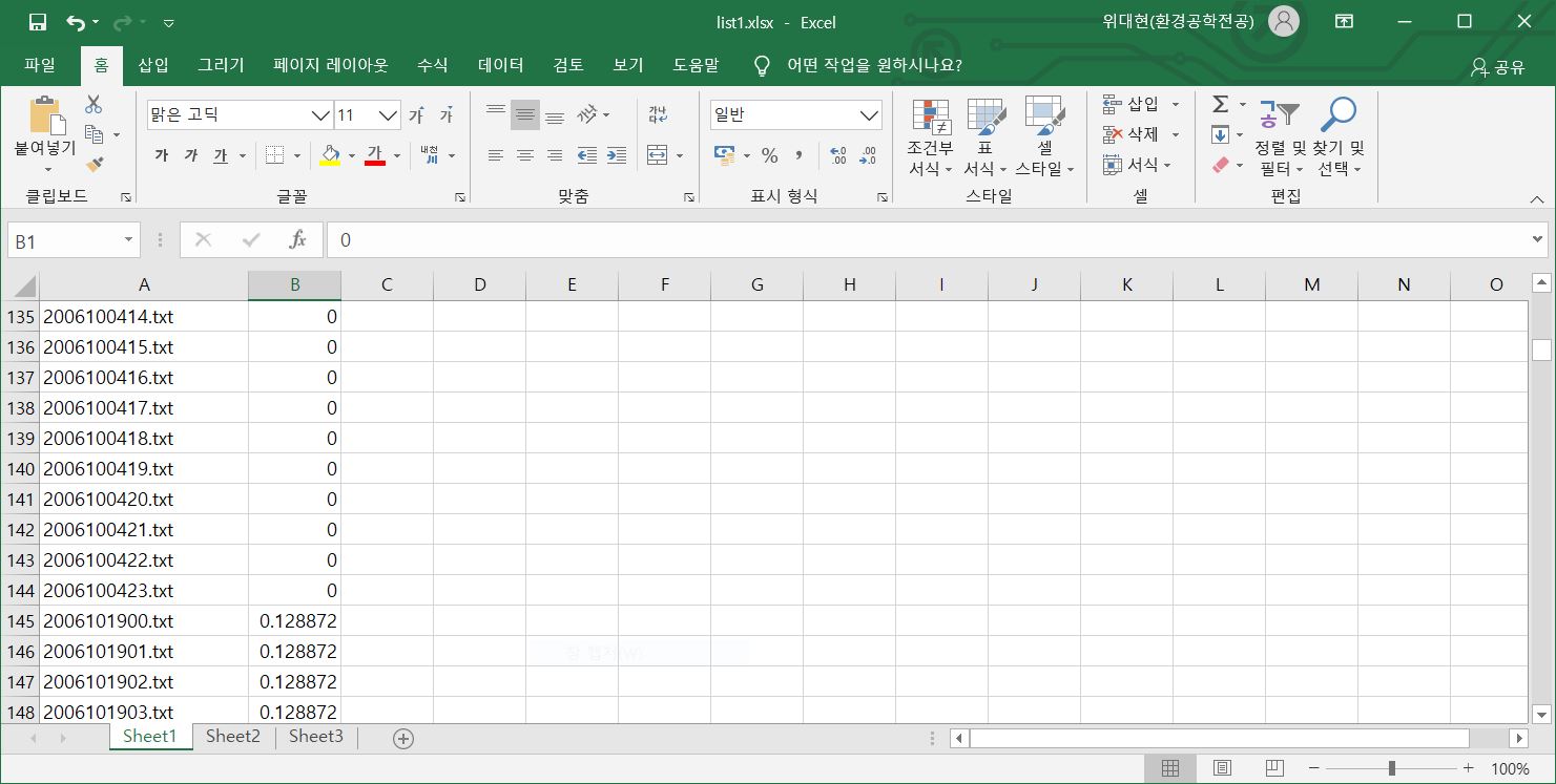
There may be cases where one measurement of pollutant concentration corresponds to many backward trajectories simultaneously. A typical duration of continuous sampling is 1 day, i.e., 24 hours, and one may want to create 24 trajectories for each hour as the sampling continues. There are two ways of dealing with such cases. First, one can input the same concentration for all of the corresponding backward trajectories, as shown in the figure above. This is a usual way with which a PSCF is obtained, but it is not really the best practice. The reason is simple. The underlying assumption behind such a practice would be that the air parcels of all the backward trajectories are equally carrying the same amount of the pollutant in them, which is clearly not true. Rather, a better way of interpretation is that the air parcels carry various amounts of the pollutant and that they all accumulate to reach the measured concentration. Thus, the average of the concentrations corresponding to all the 24 backward trajectories that arrive during the duration of sampling is the concentrarion measured at the site on that day. For the present script, one can construct the "trajectory and concentration data" file as shown in the following figure to interpret the data in this way. The first trajectory corresponds to a nonnegative concentration value in the neighboring cell on the right, which is interpreted as the average concentration value, and the other corresponding successive trajectories are given a negative value, which indicates that these trajectories are all associated with the nonnegative value given to the first trajectory. 

Another example of "trajectory and concentration data" file. One measured concentration is considered as the average of the concentrations from multiple backward trajectories. 

 

Step 2. Preparing the Script File

The main driver script is cPSDF.m, which should be run from the command line of MATLAB/Octave. The file has a section specifying input parameters, as shown in the following figure.

The section for input parameters in cPSDF.m.

Each parameter is described in the following.

 

% TRAJECTORY AND CONCENTRATION DATA FILE (xlsx)
  filenameTrajConc='trajectories/list.xlsx';

→ Specification of the "trajectory and concentration data" file. In this example, the file is located at the subdirectory "trajectories". 

 

% DIRECTORY CONTAINING TRAJECTORY FILES
directoryTraj='trajectories'; % WITHOUT THE LAST SLASH.

→ Specification of the location of the backward trajectory files. In this example, these files are located at the subdirectory "trajectories".

 

% OUTPUT FILE FOR PSDF VALUES (xlsx)
filenameOutput='outPSDF.xlsx';

→ Specification of the output file. This file will provide the PSDF values at each grid point.

 

% HYPERPARAMETERS
corLengthScale=.5; % CORRELATION LENGTH SCALE; DEGREE LAT/LONG; 
                   % TYPICALLY EQUAL TO THE CELL SIZE
r=0.5; % 0<r<1; DEFAULT ANSATZ: r=0.5 (EQUIPARTITIONING OF VARIANCE)

→ Specification of hyperparameters. The spatial correlation length scale is typically taken as 0.5 degree latitude/longitude, which is a length scale widely used for similar spatial analysis of air pollution sources. The parameter r controls the signal-to-noise ratio. If you are confident that your data set is well described by the statistical model, take a small value like 0.1. If you are unsure, a default value of 0.5 is recommended, which results in equipartitioning of variance over the signal part and the noise part.  

 

% DURATION OF BACKWARD TRACKING 
DTracking=72; % HOURS OF BACKWARD TRACKING

→ The length of backward tracking. It must be equal to the hours of the backward tracking assigned during the generation of the HYSPLIT backward trajectory data set.

 

% CELL SPEC
Nx=60;
xmin=115;
xmax=135;
Ny=50;
ymin=30;
ymax=45;

→ Specification of the grid for visualization. x corresponds to longitude, and y to latitude.

 

% SKI GRID SPEC
NGx=150;
NGy=121;

→ Specification of the interpolation grid for the SKI scheme. A grid denser than that for visualization is recommended.

 

% A MINOR NUMERICAL PARAMETER FOR INTEGRATION
% MOSTLY DO NOT HAVE TO MODIFY.
nFactor=3;

→ A numerical parameter that controls the density of uniform quadrature points in integration. Usually, users do not have to modify this parameter.

 

The remaining part of the section is not essentially important for simply running the script, and does not have to be modified in usual cases.

 

Step 3. Running the Script File

Since we are using the .xlsx format as the "trajectory and concentration data" file, Octave users must load the IO package before running the script cPSDF.m ( https://octave.sourceforge.io/io/index.html ). Time is mostly being consumed during the generation of the interpolation matrices and that of the correlation matrices. If successful, one will get a figure with PSDF values as shown in the following figure, and the output will be saved as the output file specified in the cPSDF.m.

A screenshot of an example run of cPSDF on Octave

 

History

> AUG 13, 2023
THE CODE NOW FINDS OUT THE LOCATION OF THE LINE "1 PRESSURE" AUTOMATICALLY WHEN A TRAJECTORY FILE IS PARSED. IN THE PREVIOUS VERSION, THE CODE TRIES TO READ AFTER 9 LINES WHICH MAY NOT BE ALWAYS THE RIGHT LOCATION TO START.

 

Correspondence

Questions and comments should be addressed to:

 

Daehyun Wee, Sc.D.

Associate Professor

Department of Environmental Science and Engineering

Ewha Womans University

Seoul, Republic of Korea 

dhwee@ewha.ac.kr

 

References

[1] In Sun Kim, Yong Pyo Kim, and Daehyun Wee, Potential Source Density Function: A New Tool for Identifying Air Pollution Sources, Aerosol and Air Quality Research, Vol. 22, 210236 (2022). (Open Access)
https://doi.org/10.4209/aaqr.210236 

[2] Andrew Wilson and Hannes Nickisch, Kernel Interpolation for Scalable Structured Gaussian Processes (KISS-GP), Proceedings of the 32nd International Conference on Machine Learning, PMLR 37:1775-1784, 2015.
proceedings.mlr.press/v37/wilson15.html

[3] Stein, A.F., Draxler, R.R, Rolph, G.D., Stunder, B.J.B., Cohen, M.D., and Ngan, F., (2015). NOAA's HYSPLIT atmospheric transport and dispersion modeling system, Bull. Amer. Meteor. Soc., 96, 2059-2077.
dx.doi.org/10.1175/BAMS-D-14-00110.1

[4] Rolph, G., Stein, A., and Stunder, B., (2017). Real-time Environmental Applications and Display sYstem: READY. Environmental Modelling & Software, 95, 210-228.
doi.org/10.1016/j.envsoft.2017.06.025

 

00MATLAB_cPSDF_Version20230813.zip

2.81MB